The Development of Power System Load Models Using PMU Data
Shanshan Liu with adviser Peter W. Sauer
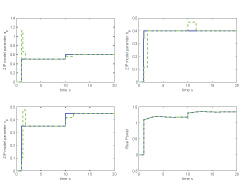
Figure 31 Parameter estimation result from LMA for static ZIP load model (blue line is the actual value and green line the estimation).
Power system load representation has a significant impact on power system analysis and control results. Unlike generators, excitation systems and transformers, which are devices, loads evolve with time, making the task of developing standard load model structure rather challenging. A phasor measurement unit (PMU) provides instant system data; hence it is possible to update the load model simultaneously to give a better understanding of the power system.
Load modeling includes two tasks: determining a suitable load model structure and deriving the parameter values for the associate load model. We will start from the constant impedance-current-power (ZIP) and static exponential models, which are routinely used in simulation studies. Then we will extend the results to other load structures and dynamic forms. The Levenberg-Marquardt algorithm (LMA), a robust method for nonlinear least-squares problems, will be used in this project.
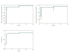
Figure 32 Parameter estimation result from LMA for static exponential load model (blue line is the actual value and green line the estimation).
For the ZIP model (see Figure 31), V0, P0 and Q0 are the values at the initial conditions of the system for the study, and the coefficients ap, bp, cp and aq, bq, cq are the parameters of the model. In this experiment, the load parameters ap, bp, cp and aq, bq, cq are changed at 1s from (0 0 0) to (0.5 0.4 0.35), and changed again at 10s to (0.6 0.4 0.45).
For the static exponential load model (see Figure 32), the parameters are as, bs, and the values of the active and reactive power, P0 and Q0, at the initial conditions. In this experiment, the parameters,(P0, as) are changed at 1s to (1.25 1.2) and changed again at 10s to (1.35 1.3).